Today’s goal is to construct development environment for data analytics and machine learning with Anaconda.
What is Anaconda?
Anaconda is open source Python distribution for data science. You can see the list of package lists here.
the open-source Individual Edition (Distribution) is the easiest way to perform Python/R data science and machine learning on a single machine. Developed for solo practitioners, it is the toolkit that equips you to work with thousands of open-source packages and libraries.
Access the websiteanaconda.com/products/individual and click “Download” button to download the installer of the edition that you want.
Start the installer and click “Continue”.
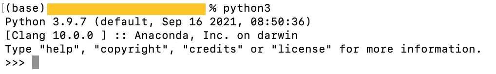
Check if anaconda is completely installed with terminal.
Start Anaconda Navigator
Start applications > Anaconda-Navigator.
Create virtual environment
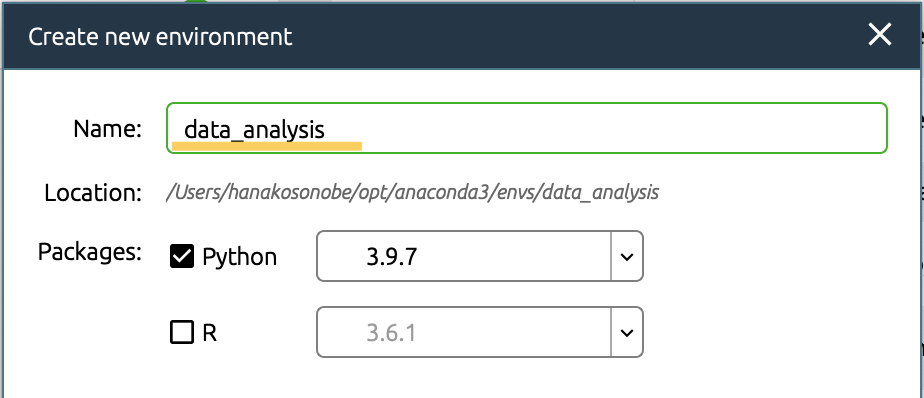
Click Environments and create new environment.
I named new environment “data_analysis”.
Install libraries or modules with conda
Conda is an open source package management system and environment management system.
Open terminal in the environment where you want to install libraries.
Then put the “conda install” command to install libraries. For example, I installed pytorch in the “pytorch” environment. The option “-c” is the channel (What is a “conda channel”?).
conda install pytorch torchvision -c pytorch
Start Application
Select environment what you want to use and install or launch application.
I launched “Jupyter notebook” and check that “pythorch” library is installed successfully.
#source code
a = 1.2
b = 2.4
c = 3.6
print(a + b == c)
False
GOAL
To understand the mechanism of the internal representation of integer and float point in computer.
Binary Number
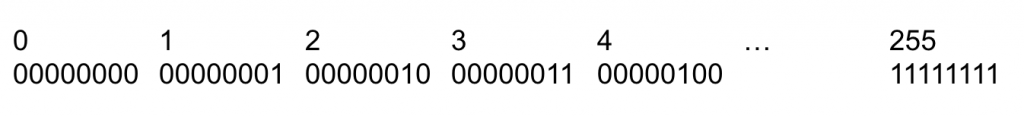
Numbers are represented as binary number in computer.
Unsigned int
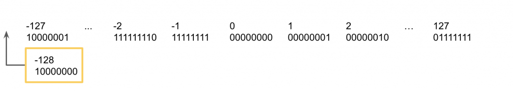
Signed int: Two’s Complement notation
What is complement?
Complement has two definition. First, complement on n of a given number can be defined as the smallest number the sum of which and the given number increase its digit. Second, it is also defined as the biggest number the sum of which and the given number doesn’t increase its digit. In decimal number, the 10’s complement of 3 is 7 and the 9’s complement of 3 is 6. How about in binary number?
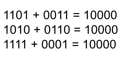
One’s complement
One’s complement of the input is the number generated by reversing each digit of the input from 0 to 1 and from 1 to 0.
Two’s complement
Two’s complement of the input is the number generated by reversing each digit of the input, that is one’s complement, plus 1. Or it can be calculated easily by subtracting 1 from the input and reverse each digit from 1 to 0 and from 0 to 1.
The range that can be expressed in two’s complement notation
The range is asymmetric.
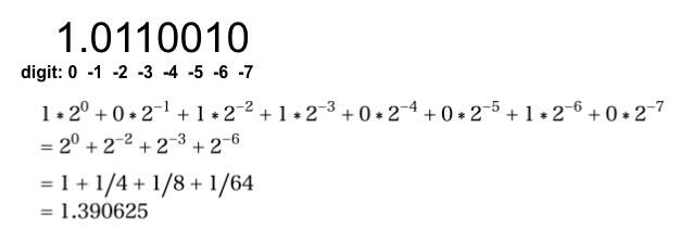
Floating point
The following is the way to represent floating point number in computer.
The digit is limited and this means that the floating point can’t represent all the decimals in continuous range. Then the decimals are approximated to closest numbers.
Why float(1.2)+float(2.4) is not equal to float(3.6)?
In computers float number can’t have exactly 1.1 but just an approximation that can be expressed in binary. You can see errors by setting the number of decimal places bigger.
#source code
a = 1.2
b = 2.4
c = 3.6
print('{:.20f}'.format(a))
print('{:.20f}'.format(b))
print('{:.20f}'.format(c))
print('{:.20f}'.format(a+b))
*You can avoid this phenomena by using Decimal number in python.
from decimal import *
a = Decimal('1.2')
b = Decimal('2.4')
c = Decimal('3.6')
print(a+b == c)

print('{:.20f}'.format(a))
print('{:.20f}'.format(b))
print('{:.20f}'.format(c))
print('{:.20f}'.format(a+b))
ANOVE is is a method of statistical hypothesis testing that determines the effects of factors and interactions, which analyzes the differences between group means within a sample. Details will be longer. Please see the following site.
One-way ANOVA is ANOVA test that compares the means of three or more samples. Null hypothesis is that samples in groups were taken from populations with the same mean.
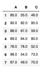
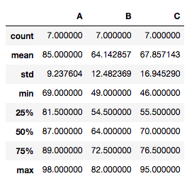
Implementation
The following is implementation example of one-way ANOVA.
Import Libraries
Import libraries below for ANOVA test.
import pandas as pd
import numpy as np
import scipy as sp
import csv # when you need to read csv data
from scipy import stats as st

import statsmodels.formula.api as smf
import statsmodels.api as sm
import statsmodels.stats.anova as anova #for ANOVA
from statsmodels.stats.multicomp import pairwise_tukeyhsd #for Tukey's multiple comparisons
csv_line = []
with open('test_data.csv', ) as f:
    for i in f:
        items = i.split(',')
        for j in range(len(items)):
            if '\n' in items[j]:
                items[j] =float(items[j][:-1])
            else:
                items[j] =float(items[j])
        print(items)
        csv_line.append(items)
The smaller the p-value, the stronger the evidence that you should reject the null hypothesis. When statistically significant, that is, p-value is less than 0.05 (typically ≤ 0.05), perform a multiple comparison.
Tukey’s multiple comparisons
Use pairwise_tukeyhsd(endog, groups, alpha=0.05) for tuky’s HSD(honestly significant difference) test. Argument endog is response variable, array of data (A[0] A[1]… A[6] B[1] … B[6] C[1] … C[6]). Argument groups is list of names(A, A…A, B…B, C…C) that corresponds to response variable. Alpha is significance level.
def tukey_hsd(group_names , *args ):
    endog = np.hstack(args)
    groups_list = []
    for i in range(len(args)):
        for j in range(len(args[i])):
            groups_list.append(group_names[i])
    groups = np.array(groups_list)
    res = pairwise_tukeyhsd(endog, groups)
    print (res.pvalues) #print only p-value
    print(res) #print result
print(tukey_hsd(['A', 'B', 'C'], tdata['A'], tdata['B'],tdata['C']))
>>[0.02259466 0.06511251 0.85313142]
 Multiple Comparison of Means - Tukey HSD, FWER=0.05
=====================================================
group1 group2 meandiff p-adj   lower    upper  reject
-----------------------------------------------------
     A      B -20.8571 0.0226 -38.9533 -2.7609   True
     A      C -17.1429 0.0651 -35.2391  0.9533  False
     B      C   3.7143 0.8531 -14.3819 21.8105  False
-----------------------------------------------------
None
Supplement
If you can’t find ‘pvalue’ key, check the version of statsmodels.
To do chi-square test and residual analysis in R. If you want to know chi-square test and implement it in python, refer “Chi-Square Test in Python”.
Source Code
> test_data <- data.frame(
  groups = c("A","A", "B", "B", "C", "C"),
  result = c("success", "failure", "success", "failure", "success",
 "failure"),
  number = c(23, 100, 65, 44, 158, 119)
)

> test_data
groups  result number
1      A success     23
2      A failure    100
3      B success     65
4      B failure     44
5      C success    158
6      C failure    119

> cross_data <- xtabs(number ~ ., test_data)
> cross_data
      result
groups failure success
     A     100      23
     B      44      65
     C     119     158

> result <- chisq.test(cross_data, correct=F)
> result
	Pearson's Chi-squared test

data:  cross_data
X-squared = 57.236, df = 2, p-value = 3.727e-13

> reesult$residuals
      result
groups   failure   success
     A  4.571703 -4.727030
     B -1.641673  1.697450
     C -2.016609  2.085125

> result$stdres
      result
groups   failure   success
     A  7.551524 -7.551524
     B -2.663833  2.663833
     C -4.296630  4.296630

> pnorm(abs(result$stdres), lower.tail = FALSE) * 2
      result
groups      failure      success
     A 4.301958e-14 4.301958e-14
     B 7.725587e-03 7.725587e-03
     C 1.734143e-05 1.734143e-05
functions
xtabs
xtabs() function is a function to create a contingency table from cross-classifying factors that contained in a data frame. “~” is the formula to specify variables that serve as aggregation criteria are described. And “~ .” means that this function use all variables (groups+result).
chisq.test
chisq.test() function is a function to return the test statistic, degree of freedom and p-value. The argument “correct” is continuity correction and set “correct” into F to suppress the continuity correction.
reesult$residuals
$residuals return standardized residuals.
result$stdres
$stdres return adjusted standardized residuals.
pnorm(abs(result$stdres), lower.tail = FALSE) * 2
This calculates p-value of standardized residuals.
Chi-square test which means “Pearson’s chi-square test” here, is a method of statistical hypothesis testing for goodness-of-fit and independence.
Goodness-of-fit test is the testing to determine whether the observed frequency distribution is the same as the theoretical distribution. Independence test is the testing to determine whether 2 observations that is represented by 2*2 table, on 2 variables are independent of each other.
Details will be longer. Please see the following sites and document.
The following is implementation for chi-square test.
Import libraries
import numpy as np
import pandas as pd
import scipy as sp
from scipy import stats
Data preparing
gourp A
group B
group C
success
23
65
158
failure
100
44
119
success rate
0.187
0.596
0.570
chi_square_data.csv
A,B,C
23,65,158
100,44,119
Read and Set Data
csv_line = []
with open('chi_square_data.csv', ) as f:
    for i in f:
        items = i.split(',')
        for j in range(len(items)):
            if '\n' in items[j]:
                items[j] =float(items[j][:-1])
            else:
                items[j] =float(items[j])
        csv_line.append(items)
group = csv_line[0]
success = [int(n) for n in csv_line[1]]
failure = [int(n) for n in csv_line[2]]

groups = []
result =[]
count = []
for i in range(len(group)):
    groups += [group[i], group[i]] #['A','A', 'B', 'B', 'C', 'C']
    result += ['success', 'failure'] #['success', 'failure', 'success', 'failure', 'success', 'failure']
    count += [success[i], failure[i]] #[23, 100, 65, 44, 158, 119]

data =  pd.DataFrame({
    'groups' : groups,
    'result' : result,
    'count' : count
})
cross_data = pd.pivot_table(
    data = data,
    values ='count',
    aggfunc = 'sum',
    index = 'groups',
    columns = 'result'
)
print(cross_data)
>>result  failure  success
groups
A           100       23
B            44       65
C           119      158
The expected frequencies, based on the marginal sums of the table.
The smaller the p-value, the stronger the evidence that you should reject the null hypothesis. When statistically significant, that is, p-value is less than 0.05 (typically ≤ 0.05), the difference between groups is significant.
ANOVA(analysis of variance) is a method of statistical hypothesis testing that determines the effects of factors and interactions, which analyzes the differences between group means within a sample. Details will be longer. Please see the following site.
One-way ANOVA is ANOVA test that compares the means of three or more samples. Null hypothesis is that samples in groups were taken from populations with the same mean.
Implementation
The following is implementation example of paired one-way ANOVA.
Import Libraries
Import libraries below for ANOVA test.
import statsmodels.api as sm
from statsmodels.formula.api import ols
import pandas as pd
import numpy as np
import statsmodels.stats.anova as anova
csv_line = []
with open('test_data.csv', ) as f:
    for i in f:
        items = i.split(',')
        for j in range(len(items)):
            if '\n' in items[j]:
                items[j] =float(items[j][:-1])
            else:
                items[j] =float(items[j])
        print(items)
        csv_line.append(items)
aov=anova.AnovaRM(df, 'Point','Subjects',['Conditions'])
result=aov.fit()

print(result)

>>                 Anova
========================================
           F Value Num DF  Den DF Pr > F
----------------------------------------
Conditions  5.4182 2.0000 12.0000 0.0211
========================================
The smaller the p-value, the stronger the evidence that you should reject the null hypothesis. When statistically significant, that is, p-value is less than 0.05 (typically ≤ 0.05), perform a multiple comparison. This p value is different between paired ANOVA and unpaired ANOVA.
Tukey’s multiple comparisons
Use pairwise_tukeyhsd(endog, groups, alpha=0.05) for tuky’s HSD(honestly significant difference) test. Argument endog is response variable, array of data (A[0] A[1]… A[6] B[1] … B[6] C[1] … C[6]). Argument groups is list of names(A, A…A, B…B, C…C) that corresponds to response variable. Alpha is significance level.
def tukey_hsd(group_names , *args ):
    endog = np.hstack(args)
    groups_list = []
    for i in range(len(args)):
        for j in range(len(args[i])):
            groups_list.append(group_names[i])
    groups = np.array(groups_list)
    res = pairwise_tukeyhsd(endog, groups)
    print (res.pvalues) #print only p-value
    print(res) #print result
print(tukey_hsd(['A', 'B', 'C'], tdata['A'], tdata['B'],tdata['C']))
>> [0.02259466 0.06511251 0.85313142]
 Multiple Comparison of Means - Tukey HSD, FWER=0.05
=====================================================
group1 group2 meandiff p-adj   lower    upper  reject
-----------------------------------------------------
     A      B -20.8571 0.0226 -38.9533 -2.7609   True
     A      C -17.1429 0.0651 -35.2391  0.9533  False
     B      C   3.7143 0.8531 -14.3819 21.8105  False
-----------------------------------------------------
None