A non-hierarchical procedure for re-synthesis of complex textures
I’ve read “A non-hierarchical procedure for re-synthesis of complex textures“. REFERENCE: Image Texture Tools: Texture Synthesis, Texture Transfer, and Plausible Restoration.
Texture re-synthesis
In this paper, texture re-synthesis means the name of the technique to generate output texture with a similar pattern to the one of input image.
Novelty of the study
This work propose a method for synthesizing an image with the same texture as a given input image. In this method, a plausible value for dot in output image is selected from input image. Important point is the order to select dot to transfers complex features of the input image to the output image.
Method
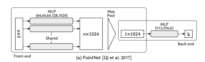
overview
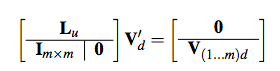
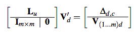
Select pixels in output image and set a value from pixels in input image. Pixel value estimation depends on entropy, amounts of information, of pixels in the input image. To measure how closely a patch from the input image matched one from the output image, distance function below is used. In other word, the distance function indicates the plausibility of the selected pixel.
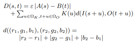
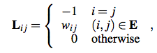
t: pixel from the output image
A, B: random function
Ωk: offset(the range of the patch)
K(u): Weighting given to a particular offset
I(s+u): rgb value of the pixel s+u
O(t+u): rgb value of the pixel t+u
- Find empty location in the output image with the highest priority.
- Choose a pixel from the input image to place in the location.
- Update priorities of empty neighboring location based on the new pixel value
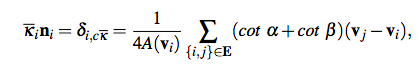
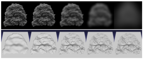
Analysis of pixel interrelationships in the input image
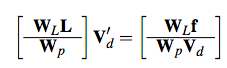
To select important pixel with large amount of information, define the number of bits of information G(s, u). The prioritization weighting and the order of pixel addition can be decided by using this G(s, u). Refer the original paper to derive G(s, u) and weightings from RGB data of the input image.
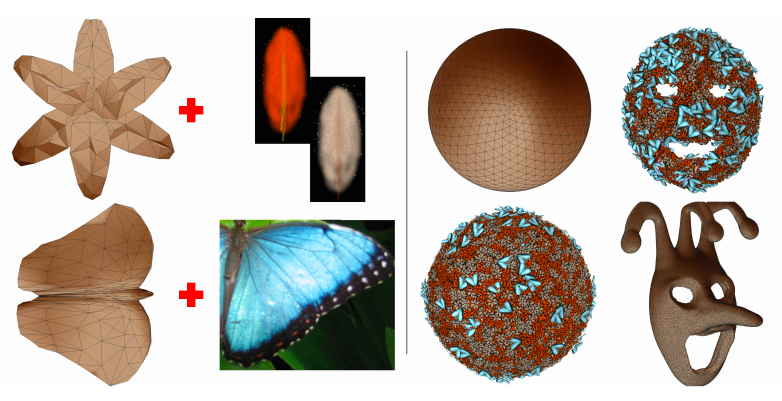
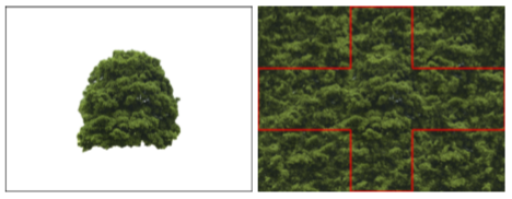
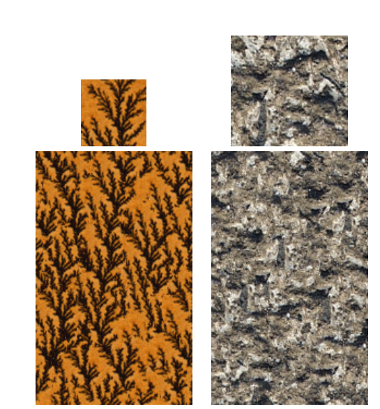
Result
In this paper seven neighborhood of pixels was used. It takes 4.5 minutes and 6.5MB of memory to produce on a 8000Mhz Pentium2.
You can see more result and application in the original paper.